Excel percentage formulas can get you through problems large and small every day—from determining sales tax (and tips) to calculating increases and decreases. We’ll walk through several examples below: turning fractions to percentages; backing sales tax out of totals; percentage of total; percentage increase or decrease; percentage of completion; and percent ranking (percentile).
How to turn fractions into percentages
Percentages are a portion (or fraction) of 100. The math to determine a percentage is to divide the numerator (the number on top of the fraction) by the denominator (the number on the bottom of the fraction), then multiply the answer by 100. For example, the fraction 6/12 turns into a decimal like this: 6 divided by 12 (which equals 0.5) times 100 equals 50 percent.
In Excel, you don’t need a formula to convert a fraction to a percent—just a Format change. For example:
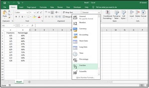
1. Enter 10 fractions in column A (from A2 through A11). (Note: Excel automatically reduces fractions to their lowest terms, such as changing 6/10 to 3/5.)
Because the Excel default is decimal, you’ll need to highlight the range and format it for Fractions. Here’s how:
2. Copy the fractions in column A to Column B.
3. Highlight that range and go to the Home tab. Select Percentage from the dropdown list in the Number Formats field.
 JD Sartain / IDG
How Excel converts fractions to percentages
NOTE: You can also select Format Cells from the Format button in the Cells group.
How to back sales tax out of totals
Some companies sell products with the sales tax included, then just back the tax out for their payments to the IRS. Calculate this by dividing the “sticker” price (or receipt total) by 1.0 plus the sales tax rate. For example, if you paid $50 for a lamp and the local sales tax rate is 9%, divide $50 by 1.09. The actual retail price before sales tax is $45.87, and the sales tax is $4.13. To check your answer, just add the two numbers together, or multiply $45.87 by 9%.
Using a calculator to do this for just one item is fine, but if you’re pulling sales taxes out of your weekly or monthly product sales, you only have to enter the formula once, then copy it throughout your entire sales and inventory spreadsheet.
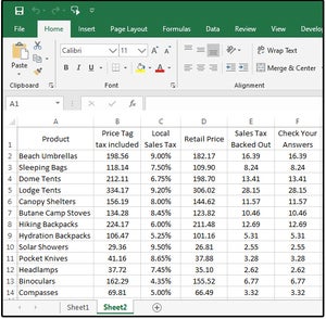
1. Enter a dozen or so products in column A (from A2 through A14).
2. Next, enter the corresponding receipt total price (tax included) in column B (from B2 through B14).
3. In columns C2 through C14, enter several arbitrary sales tax percentages (so you have some different numbers to play with). Be sure to enter some decimal/fractional percentages such as 4.75%, because most sales taxes are not whole numbers.
4. Enter this two-step formula in cell D2: =SUM(B2/(C2+1)) . The object here is to convert the tax percentage to the whole number divisor (e.g., 9% to 1.09), and then divide the receipt total price ($198.56) by the whole number divisor (1.09) to get the correct retail price (before taxes) of $182.17.
5. Copy the formula from D2 down to D14.
6. In cell E2, subtract D2 from B2 to get the actual “backed-out” sales taxes (for the IRS): =SUM(B2-D2). Copy the formula from E2 down through E14.
7. To double-check your answers, enter this formula in F2 through F14: =SUM(D2*C2). If the columns E and F match, your data is correct.
 JD Sartain / IDG
Back out the sales tax from the receipt’s total
How to get percentage of totals
If you’re self-employed or have an office in your home, one method the IRS uses to determine your deductions (for the office portion of your rent, utilities, household maintenance costs, etc.) is to subtract the square footage of the office from the home’s total square footage. You can claim a percentage of those totals. The math for this one begins with dividing the office square footage by the home’s total square footage, then calculating the overhead based on that percentage.
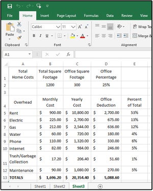
1. Across the top, enter your home’s total square footage in cell B2.
2. Enter the total square footage of your office in C2.
3. Enter this formula in cell D2: =SUM(C2/B2) to determine the office’s percentage of square feet (in this case, 25%).
4. Enter your home and office overhead items in column A (rent, electricity, etc.)
5. Enter the monthly cost of each item in column B.
6. Enter this formula in cells C5 through C12: =SUM(B5*12) . This gives you the yearly totals.
7. Enter this formula in cells D5 through D12: =SUM(C5*$D$2). The cell address D2 must be absolute. Use function key F4 to add the dollar signs that make the formula absolute, so each cell in column D is multiplied by D2.
8. Total columns B, C, and D on row 13.
Now you can see how much you spent on monthly and yearly overhead for the entire house and for the office only. Cell D13 shows your total home office deduction ($5,088.60).
9. To calculate the percent of the total overhead by item, enter this formula in E5 through E12: =SUM(B5/$B$13). Use these percentages to determine if your monthly/yearly overhead is within normal business practices.
![003 percentage of totals for home office deduction and overhead]() JD Sartain / IDG
JD Sartain / IDG
 JD Sartain / IDG
Percentage of totals for home office deduction and overhead
How to figure out percentage of price increase or decrease
For most businesses, especially in retail, owners and managers like to know the percentages of increase and decrease for just about everything, from sales to salaries. Use the following formulas to calculate the percentages of increase and decrease in your company.
Imagine you’ve created a workbook with a spreadsheet tab called “Increase-Decrease.” Another spreadsheet tab called “SalesTax” includes Retail Sales Price data.
1. Enter a dozen or so product items in column A of Increase-Decrease (or just copy the same items used in the spreadsheet from part A above).
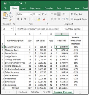
2. Enter the quantities sold of each item in columns B and D.
3. Enter this formula in the “Jan Sales” column (C2 through C14): =SUM(SalesTax!D2*’Increase-Decrease’!B2). This formula tells Excel to multiply the Retail Sales Price in column D of the spreadsheet called SalesTax by the quantity amounts in column B of the spreadsheet where our cursor currently resides, Increase-Decrease.
4. Enter this formula in the “Feb Sales” column (E2 through E14): =SUM(SalesTax!D2*’Increase-Decrease’!D2).
5. Next, enter this formula in F2: =SUM(E2-C2)/C2.
The positive numbers show the sales increase percentage between January and February, while the negative numbers represent the percentage of decrease in sales.
 JD Sartain / IDG
Percentages of increase and/or decrease in product sales by month
How to calculate percentage of a task or project completion
Instead of spending money on a project management software program, use the following formulas to manage the planning and flow of each project with the percentage of completion at specified intervals.
1. In column A, enter the names for half a dozen projects (in progress).
2. In columns B and C, enter the Start and End Dates of each project.
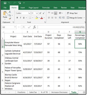
3. To determine the project completion (so far), subtract the Start Date from the End Date. Enter this formula in column D2 through D7: =SUM(C2-B2).
4. In column E, enter the number of days completed so far. This is the only column of data that you will ever change; for example, once a day (or week), access this spreadsheet and modify the data in this column to get accurate conclusions in columns F and G (days left and percentage completed).
5. To get the number of days left in each project, enter this formula in column F2 through F7: =SUM(D2-E2). This numbers will continually change based on the number data in column E (number of days completed).
6. And last, enter this formula to get the percentage of the task/project completed, so far: =SUM(E2/D2).
 JD Sartain / IDG
Calculate the percentage of a task/project completed
How to do percent ranking
Imagine that you have dozens of people applying for national parks and forestry jobs. From the resumes and the initial interviews, they all seem to be equally qualified. However, they must meet some minimum qualifications that are not generally indicated on resumes, such as how to safely remove porcupine quills from a dog’s face and neck.
The solution: Give the applicants a skills test, and use Excel’s PERCENTRANK.EXC function to determine the ranking percentile of each applicant.
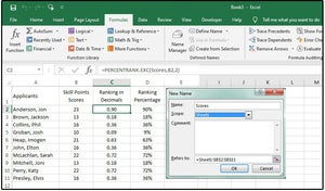
Enter 10 applicant names in cells A2:A11. Enter the skill points (scores) between 10 and 100 for each applicant in cells B2:B11 and then name the range.
Select/highlight cells B2:B11. Select Formulas > Define Name > Define Name and enter the word Scores in the Name field box. Click the arrow beside the Scope field box and choose Sheet1 from the list to identify the range location. Notice the Refers To field box contains the cell addresses of the highlighted/selected range. If the range is incorrect, click the red arrow on the right and enter the correct range addresses, or re-select the correct cells, and then click OK.
NOTE: You must define and name the range of the “array” for the formula to work.
Next, enter the following formula in cell C2: =PERCENTRANK.EXC(Scores,B2,2) where Scores equals the range name, B2 is the first value in the range, and 2 means display two decimal places.
Copy and paste the formula down through cell C11. Notice that the only piece of the function that changes as you cursor down through list is the cell address (B2, B3, B4, etc.).
You can format the decimal numbers as a percent for easier viewing. Just highlight the range and select Percent from the Format Cells dialog. Or Copy column C and choose Paste > Special > Values to replicate the text in column D. Note, however, that if you change any of the values in column B, you will have to repeat the Copy-Paste-Special-Values step.
To ensure the values are always updated and current, enter the following formula in D2: =VALUE(C2), then copy and paste down through D11.
Notice that three applicants have 22 points with a ranking percentile of 72 percent. This means that their scores are greater than or equal to 72 percent of all the test scores. If you change the first score from 22 to 23, the ranking percentage jumps to 90 percent, because this score is now in the top 90th percentile of all the test scores.
 JD Sartain / IDG
Use the PERCENTRANK.EXC function to determine the ranking percentiles of a selected group
Note: When you purchase something after clicking links in our articles, we may earn a small commission. Read our affiliate link policy for more details.
Stay connected with us on social media platform for instant update click here to join our Twitter, & Facebook
We are now on Telegram. Click here to join our channel (@TechiUpdate) and stay updated with the latest Technology headlines.
For all the latest Technology News Click Here
For the latest news and updates, follow us on Google News.
Denial of responsibility! NewsAzi is an automatic aggregator around the global media. All the content are available free on Internet. We have just arranged it in one platform for educational purpose only. In each content, the hyperlink to the primary source is specified. All trademarks belong to their rightful owners, all materials to their authors. If you are the owner of the content and do not want us to publish your materials on our website, please contact us by email – [email protected]. The content will be deleted within 24 hours.